Conditional Formatting - Using Formula

Using Formula to determine which cells to format

There are many options to choose from when using conditional formatting, however at times we will need to use formula to manipulate our conditions further.

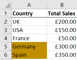
An example of using a formula to determine which cells to format, would be to format cells in Column A if the relative cell in column B was greater than 200. (Please see below example)

To achieve this:

1. Select the cells you wish to format, in this example that would be A2:A6, becasue we want the country name cell to fill gold if it meets the above criteria.

2. Select the Home tab, and then select the Conditional Formatting Command from the Styles Group. Select New Rule...

3. Select the bottom option, use a formula to determine which cells to format
4. Type in the formula you want to use, in the example above that would be, =B2:B6 > 200
5. Select Formats, in the example that will be cell fill gold.

The New Formatting Rule Window will now look like this:

Tips:

- By default the formula will look like this: $B$2:$B$6>200 – you will need to remove the $ otherwise your formatting won’t be relative to the row it is on.

- Whilst typing your formula refrain from using the keybord arrows, this will add cells to your formula relative to the active cell you are in.

6. OK

The end result will be that any cells that contain values greater than 200, will be filled gold, as pictured below.

For more help with Conditional formatting, please look at our Excel Level 3 Courses.