Tech Tips
SQL - Comparing Multi-Table Query Styles - Part 2
Why do you need to involve a table in a query if we don’t need any columns from it you ask? Well, probably because the record set we want back from one table is dependent upon the existence of related records in another table.

Working with Multi-Table Queries That Only Require Columns From One Table
Part 1 of this series of blogs explored a number of ways of tackling a multi-table query.
Part 1 identified that sometimes choosing the right method to extract related records can be a challenge. You might be able to think of a number of ways of structuring a query to produce the same set of records, but which method should you use? I said that the answer might come from a couple of considerations:
- Which method is the most efficient and fastest?
- Which method is the easiest to understand, write and maintain?
And some of the methods listed were:
- Straight forward table JOIN
- Derived table - simple subquery
- Derived table - correlated subquery
- CROSS APPLY
- Simple subquery - nested in SELECT list and WHERE clause
- Correlated subquery - nested in SELECT list and WHERE clause
- Simple subquery in WHERE clause
- INTERSECT
The series of blogs explores three join scenarios:
- We need to retrieve/display columns from more than one of the tables involved
- We only need to retrieve/display columns from one of the tables involved
- We are looking for a common set of values between two record sets
We will use the AdventureWorks database on a SQL Server instance for our examples, but the principals laid out in this blog will apply across Azure SQL, Synapse Dedicated Pools and Fabric Warehouse. The tools used to look at execution plans will be different on these latter platforms, and the plans may look a little different in Synapse and Fabric.
In the first blog of the series we looked at multi-table queries where we need columns from more than one table to be returned in the results set.
Part 2 – Retrieving values from a single table
In part 2 of the series we look at multi-table queries where we need columns from only one of the tables involved.
Why do you need to involve a table in a query if we don’t need any columns from it you ask?
Well, probably because the record set we want back from one table is dependent upon the existence of related records in another table. For example:
- Customers who have placed orders
- Products that have been ordered
- Vehicles that have been on a call out
- Employees that have been sick
Here are six different queries to produce the same set of results. All of them display the names of employees. Employee records are stored in a table called HumanResources.Employee, but their names are not stored in this table, they are in a separate table called Person.Person. These two tables are related by a common column called BusinessEntityID in both tables.
We can see the results from the first four queries here, but the last two queries produce an identical set of records:
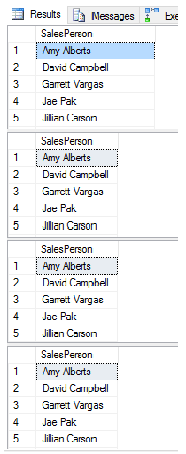
The six queries have an ORDER BY clause on them to ensure that records are returned in exactly the same order (this may not be necessary for an actual application, but helps us to verify the results sets are truly identical and like for like). Without it, although the same records are returned they may be returned in differing orders. Try it and see!
All queries also restrict the records to those relating to orders placed in 2012 only.
Working With SQL INNER Joins
The first query uses a simple INNER JOIN joining the person record to the employee record via the Primary Key/Foreign Key columns BusinessEntityID.
/*Queries where columns are only required from one table*/

--Simple join
SELECT DISTINCT FirstName + SPACE(1) + LastName AS "SalesPerson"
FROM Sales.SalesOrderHeader AS sh
	JOIN Person.Person AS p ON sh.SalesPersonID = p.BusinessEntityID
WHERE YEAR(OrderDate) = 2012
ORDER BY "SalesPerson"
Derived Table
The second query uses a derived table to retrieve the Sales.SalesOrderHeader records. A derived table is a subquery placed in the FROM clause of an outer query. The join condition between the Person.Person table and the subquery is positioned after the subquery. The subquery must be given a table name, even though it may not be referenced, which in this example is “s”.
--Derived table - simple subquery
SELECT DISTINCT FirstName + SPACE(1) + LastName AS "SalesPerson"
FROM Person.Person AS p
	JOIN
		(SELECT SalesOrderID, SalesPersonID
		 FROM Sales.SalesOrderHeader AS sh
		 WHERE YEAR(OrderDate) = 2012
		) AS s
		ON s.SalesPersonID = p.BusinessEntityID
ORDER BY "SalesPerson"
We could also have written the query with the Person.Person table being used as the basis for the derived table. This is the third query:
--Derived table - simple subquery
SELECT DISTINCT SalesPerson
		 FROM Sales.SalesOrderHeader AS sh
	JOIN
		(SELECT BusinessEntityID, FirstName + SPACE(1) + LastName AS "SalesPerson"
		 FROM Person.Person) AS p
 		 ON sh.SalesPersonID = p.BusinessEntityID
WHERE YEAR(OrderDate) = 2012
ORDER BY "SalesPerson"
The results are the same.
CROSS APPLY
The fourth query implements a CROSS APPLY statement. CROSS APPLY enables a subquery to be evaluated for every record in the table to the left of it. The join condition is placed in the WHERE clause of the subquery.
--CROSS APPLY
SELECT DISTINCT FirstName + SPACE(1) + LastName AS "SalesPerson"
FROM Person.Person AS p
	CROSS APPLY
		(SELECT SalesOrderID, SalesPersonID
		 FROM Sales.SalesOrderHeader AS sh
		 WHERE YEAR(OrderDate) = 2012
		 AND sh.SalesPersonID = p.BusinessEntityID
		) AS s
ORDER BY "SalesPerson"
A Simple Subquery
The fifth version has a subquery in the WHERE clause to restrict the results set to the person records that relate to a sales people who have taken orders, as we only wish to retrieve the name of the sales person and not any details from the order we can use a simple subquery.
--Simple subquery in WHERE clause
SELECT FirstName + SPACE(1) + LastName AS "SalesPerson"
FROM Person.Person AS p
WHERE p.BusinessEntityID IN
		(SELECT SalesPersonID
		 FROM Sales.SalesOrderHeader AS sh
		 WHERE YEAR(OrderDate) = 2012)
ORDER BY "SalesPerson"
A Correlated Subquery
The sixth version has a correlated subquery instead of a simple query and uses the WHERE EXISTS clause:
--Correlated subquery in WHERE clause
SELECT FirstName + SPACE(1) + LastName AS "SalesPerson"
FROM Person.Person AS p
WHERE EXISTS
		(SELECT SalesPersonID
		 FROM Sales.SalesOrderHeader AS sh
		 WHERE YEAR(OrderDate) = 2012
		 AND sh.SalesPersonID = p.BusinessEntityID)
ORDER BY "SalesPerson"
So which SQL JOIN method is Best?
So we ask the question again about which method is best. To answer that question we turn our attention to the Query Execution Plans.
As I mentioned in the Part 1 article, the reality is that often when we write an SQL query the database management system’s Query Optimizer may well simplify or rewrite your query to make it better, which can result in the same execution plan being produced regardless of how you structure your query.
We will see that the query plans for all six queries seen above produce exactly the same execution plan, but as stated in Part 1 it still matters what way you write the query as there are many things that influence whether a query can be simplified by the optimiser and what eventual execution plan will be used. Remember that among the top influencers are:
- The size of the tables involved
- The relative sizes of tables involved
- Columns included in the SELECT list
- WHERE clause conditions included – SARGs or not SARGs
- The use of NOT operators in WHERE clause conditions
- The existence of indexes
And remember this performance tip when writing your queries:
Always limit select lists to just the columns and expressions you require, always specify a WHERE clause when possible, avoid using NOT anywhere in a WHERE clause if possible, create indexes on columns that frequently appear in WHERE clauses.
So let’s take a look at the execution plan that all six of the above queries resulted in:
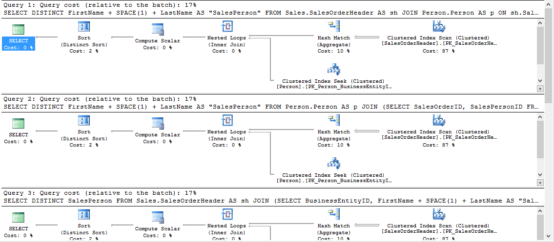
I have only shown the first two plans and the top of the third, but if you try it out, on SQL Server 2014 you will find that all six execution plans are identical (a sixth of 100% is 17% (rounded)).
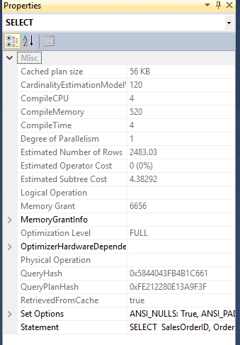
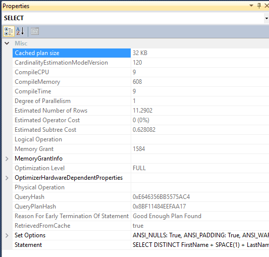
Another indicator that queries have been evaluated with the same plan is to look at the QueryPlanHash value property for each SELECT operator in the execution plan. They will often be the same. Here are the properties for Query 1:
And here are the properties for Query 2:
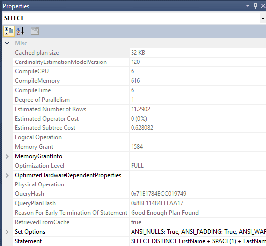
The QueryPlanHash values are both 0x8BF11484EEFAA17 and if you look at the other four plans you will find that the first four execution plans have the same value, but the last two (the subquery and correlated subquery) have a different QueryHashPlan value (although they match each other). This will be because essentially the first four queries are all forms of joins, and the last two are subqueries in a WHERE clause.
The QueryHash property, however, is different for each of the queries.
The QueryHash value is a hash of the actual SQL statement, but the QueryPlanHash is a hash of the selected plan.
Even though we have two QueryPlanHash values across the six queries the resulting execution plans are identical.
SQL Query Simplification
By looking at the plans we can see that all six were executed as an INNER JOIN. All queries involving subqueries were simplified.
So the nett effect is that each method used above has ultimately resulted in the same resource costs, but this may not always be the case.
Let’s look at an example where simplification couldn’t be carried out.
Working with SQL OUTER Joins
I have taken a similar set of six queries, but this time we are interested in records that don’t have matching records in a second table (People that are not sales people who have taken orders).
The following screen shot shows the results sets:
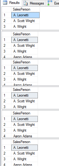
Once again each query has an ORDER BY on it to ensure the result sets are truly identical.
OUTER JOIN
The first query uses a simple OUTER JOIN joining the person record to the order record via the Primary Key/Foreign Key columns BusinessEntityID and SalesPersonID, but the WHERE clause limits the records to Person records with no corresponding SalesOrderHeader records:
--Simple outer join with outers only
SELECT FirstName + SPACE(1) + LastName AS "SalesPerson"
FROM Sales.SalesOrderHeader AS sh
	RIGHT JOIN Person.Person AS p ON sh.SalesPersonID = p.BusinessEntityID
WHERE SalesPersonID IS NULL
ORDER BY "SalesPerson"
OPTION(RECOMPILE)
This query also introduces the OPTION(RECOMPILE) which forces a query to be re-optimised every time it is executed rather than using a plan already cached.
Derived Table
The second and third queries use a derived table to retrieve the Person.Person records without matching records in Sales.SalesOrderHeader. The following example uses a LEFT JOIN:
--Derived table - simple subquery -outers only
SELECT FirstName + SPACE(1) + LastName AS "SalesPerson"
FROM Person.Person AS p
	LEFT JOIN
		(SELECT SalesOrderID, SalesPersonID
		 FROM Sales.SalesOrderHeader AS sh
		) AS s
		ON s.SalesPersonID = p.BusinessEntityID
WHERE SalesPersonID IS NULL
ORDER BY "SalesPerson"
OPTION(RECOMPILE)
The next example uses a RIGHT JOIN:
--Derived table - simple subquery - outers only
SELECT SalesPerson
		 FROM Sales.SalesOrderHeader AS sh
	RIGHT JOIN
		(SELECT BusinessEntityID, FirstName + SPACE(1) + LastName AS "SalesPerson"
		 FROM Person.Person) AS p
 		 ON sh.SalesPersonID = p.BusinessEntityID
WHERE SalesPersonID IS NULL
ORDER BY "SalesPerson"
OPTION(RECOMPILE)
OUTER APPLY
The fourth query implements an OUTER APPLY. An OUTER APPLY is the outer version of a CROSS APPLY:
--CROSS APPLY
SELECT FirstName + SPACE(1) + LastName AS "SalesPerson"
FROM Person.Person AS p
	OUTER APPLY
		(SELECT SalesOrderID, SalesPersonID
		 FROM Sales.SalesOrderHeader AS sh
		 WHERE sh.SalesPersonID = p.BusinessEntityID
		) AS s
WHERE SalesPersonID IS NULL
ORDER BY "SalesPerson"
OPTION(RECOMPILE)
Simple Subquery in WHERE Clause
The fifth query uses a simple subquery in a WHERE clause:
--Simple subquery in WHERE clause
SELECT FirstName + SPACE(1) + LastName AS "SalesPerson"
FROM Person.Person AS p
WHERE p.BusinessEntityID NOT IN
		(SELECT SalesPersonID
		 FROM Sales.SalesOrderHeader AS sh
		 WHERE SalesPersonID IS NOT NULL)
ORDER BY "SalesPerson"
OPTION(RECOMPILE)
Correlated Subquery in WHERE Clause
The sixth query uses a correlated subquery in a WHERE clause:
--Correlated subquery in WHERE clause
SELECT FirstName + SPACE(1) + LastName AS "SalesPerson"
FROM Person.Person AS p
WHERE NOT EXISTS
		(SELECT SalesPersonID
		 FROM Sales.SalesOrderHeader AS sh
		 WHERE sh.SalesPersonID = p.BusinessEntityID)
ORDER BY "SalesPerson"
OPTION(RECOMPILE)
So Which Join Is Best?
Once again we ask the question about which method is best. And once again we turn our attention to the Query Execution Plans to answer it.
We’ll take a look at the execution plans that these queries resulted in. There are actually four different plans produced by the six queries.
- Queries 1 and 3 result in an identical execution plan
- Queries 2 and 4 result in an identical execution plan
- Query 5 has a unique execution plan
- Query 6 has a unique execution plan
The execution plans are shown a little bit later on.
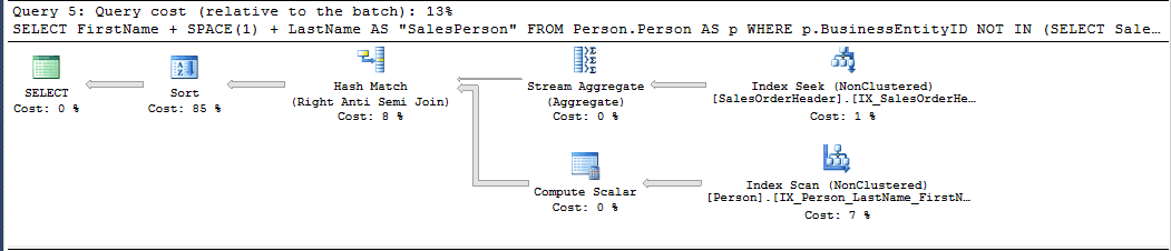
- The cheapest plan is the plan for Query 5 at a cost value of 1.56167 (13% of the batch of 6 queries).
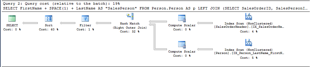
- The most expensive plan is that for queries 2 and 4 at a cost value of 2.21372 (19% of the batch of 6).
So it would seem that using a simple sub query in a WHERE clause is the best approach to this particular requirement.
We are often advised to avoid subqueries wherever possible and use joins instead, but we can see that this is not always the case.
In the first set of six queries they were all simplified to inner joins and all resulted in the same final execution plan. In the second six we can see that simplification hasn’t been possible in the last two queries. You will generally find that if you have a NOT in a WHERE clause that includes a sub query that the query cannot be simplified to a join. We can see that both query 5 and query 6 have an Anti Semi Join physical operation combining the two data streams rather than a join.
Queries 1 and 3
Here is the execution plan for queries 1 and 3:
Queries 2 and 4
Here is the execution plan for queries 2 and 4:
Query 5
Here is execution plan for query 5:
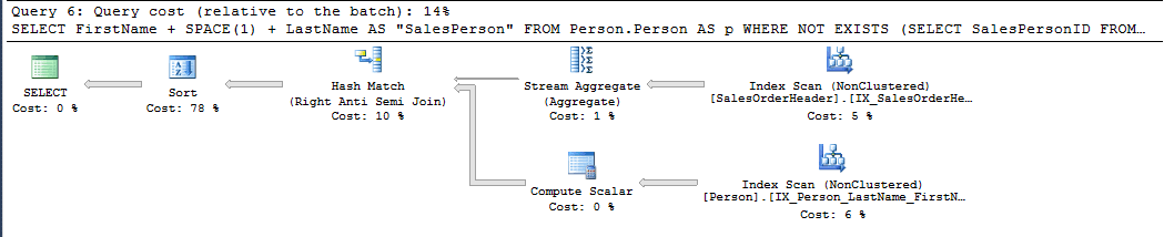
Query 6
Here is the execution plan for query 6:
Final Plans
Looking at the final plans for our six queries we can see that some changes to the way we wrote the queries have been made.
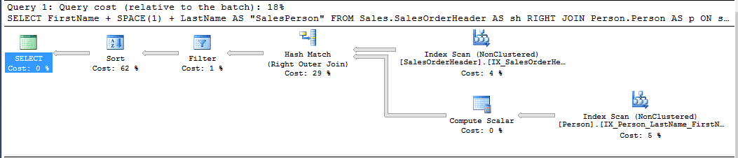
- In query 1 the resulting plan is as we wrote the query – a RIGHT JOIN, a filter for NULL SalesPersonID values and a sort.
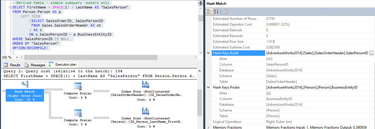
- In query 2 the LEFT JOIN we wrote has been changed to a RIGHT JOIN with the tables switched round. The Query Optimizer decides which table it will use as the Outer table (the one on the top line of the join – master) and which table it will use as the Inner table (the bottom line of the join – detail). The terms outer an inner here have nothing to do with outer joins and inner joins. For a Hash Join these tables are referred to as the Build (top one) and Probe (bottom one). The following screen shot shows the Sales.SalesOrderHeader table has been selected as the Build table and the Person.Person table has been selected as the Probe table. The optimizer will choose the smallest table as the Probe table.
- In query 3 we can see that the subquery has been simplified to a RIGHT JOIN.
- In query 4 we can see that the OUTER APPLY has been implemented as a RIGHT JOIN.
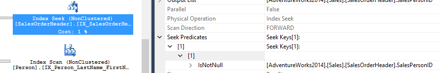
- In query 5 the optimizer has been unable to simplify the sub query to a join as there is a NOT IN clause. The resulting logical operation is a Right Anti Semi Join indicating that the sub query was retained. We can also see that an Index Seek was carried out on the SalesPersonID non clustered index. It is the only plan that has an index seek rather than a scan in it (the index was used to find a specific set of records rather than just reading every index leaf page). This has resulted in only 3806 rows being returned from the SalesOrderheader table (SalesPersonID index) as opposed to 31465 rows being returned by all the other Index Scan operations associated with the Sales. SalesOrderHeader table.
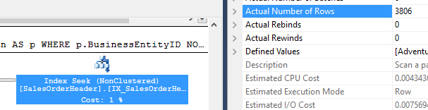
In the following screen shot we can see that the seek is filtering the NULL records out resulting in a much smaller record set to join to the Person.Person records.

- In query 6 again the optimizer has been unable to simplify the correlated sub query to a join so we see a Right Anti Semi Join operation. We can also see that the correlation between the two queries (the join) results in an Index Scan of the salesPersonID index this time with the full 31465 rows being returned. That is why this plan is slightly more expensiove than query 5. It is still, however, a better plan than queries 1 to 4.
I could go on analysing these execution plans further and digging in to the operator properties:
- Why do we have Hash Match join operations in the second six queries and Nested Loop join operations in the first six queries?
- How does SQL Server know how big the tables are?
- How does SQL Server decide whether to use an index?
- and so many more ……...
That would be too much for this article. I’ll write about them in the future.
Conclusion – Choosing the Most Efficient SQL Query
So what can we conclude?
- The optimizer does its own thing
- How we write our queries influences what the optimizer can simplify
- The sizes of our tables may result in:
- LEFT JOINS becoming RIGHT joins or vice versa
- Indexes being selected rather than table scans
- Joins are not always better than sub queries
The conclusion is that a good knowledge of how the SQL Server Optimizer works and the benefits and architecture of indexes can help you to better design your SELECT statements and achieve an optimal Query Execution Plan. So stop, think, write your queries with care and try different approaches. Inspect execution plans to see which style of query looks best!
We continue to see that there are so many factors that affect query performance and query plan selection – we identified some in Part 1 and have seen a few more in Part 2, and you are getting more of a taste of things to consider.
Do you need help in tuning poorly performing SQL queries?
We offer consultancy, training and blended solutions in SQL Server performance tuning. Take a look at our SQL Server Performance & Tuning course. Or give us a call if you think we can help you with our consultancy service.
The query optimiser varies across SQL Server on premise, Azure SQL, Synapse Dedicated Pool and Fabric Warehouse so there will be slight differences in execution plans and performance across the platforms. That said, the basic principals in assessing the mode efficient format of SQL join statements will still apply across all these platforms.
MD
Mandy Doward
Managing Director
PTR’s owner and Managing Director is a Microsoft certified Business Intelligence (BI) Consultant, with over 35 years of experience working with data analytics and BI.
Related Articles
Frequently Asked Questions
Couldn’t find the answer you were looking for? Feel free to reach out to us! Our team of experts is here to help.
Contact Us