Excel - Creating drop Down Lists in Cells

Creating A Drop Down Lists For Users to Choose From In Excel

In the following example we can see a drop list that a user can choose from when populating a Country column value.

We can see that a drop down list of countries is available when we click in one of the Country cells. We can now use the arrow keys to highlight the country we wish to select and then hit return or click on the left mouse button.

In the following screen shot we can see that Australia was selected.

It is perfectly OK to enter text into the Country cell manually, but the resulting value must match one of those list in the drop down list.

If an incorrect value is entered the following dialog pops up:

A more helpful message can be specified that indicates more clearly what the validation requirement is.

It is also possible to provide help text that is displayed as soon as a user moves into a country cell:

Adding a Validation List Rule To A Range of Cells

The first step is to create a table containing the list of possible values for the drop down. (If you are new to Excel Tables and would like to learn how to create and work with Excel Table take a look at this PTR blog article)

In the sample workbook we are using here we have a worksheet dedicated to tables used for drop down lists.

Note that Column I contains the Customer Type valid values, they have not been organised as a “Table”. You can see that there is no Table Tools Design Ribbon available when we click in one of the Customer Type cells.

If we click in any cell in the Sales Territory Country column (Column C) we will see that the Table Tools Design Ribbon is available. This is because we have created a table from cells C1 to C8.

The Table Tools Design Ribbon is selected and on the top left of the ribbon we can see that the selected table is called Countries. It is important that the list is formatted as a table as we want newly added countries to be added to the validation list automatically.

Creating The Validation List

The Data ribbon offers a Data Validation option on the Data Tools section:

Clicking on the arrow to the right of the Data Validation option displays the following options:

To add list validation to Excel Cells firstly select the range of cells that the validation list is to be available for, then select Data Validation.

Selecting Data Validation enables us to define validation rules to restrict values that a user enters into a cell.

To add a validation (drop down) list click in the drop down list for the Allow field:

Selecting List will change the dialog to offer a Source field:

The Source field can then be populated with the cell range that contains the values to be added to the List:

The above screen shot shows that rows 2 to 7 of column I on the Validation List Tables worksheet are being added to the list.

Creating a Drop Down Validation List From a Non Table List

We will take a look at creating an Excel Validation List from data not formatted as a table. We are going to add a drop down list for the Customer Type column. On our Validation List Tables worksheet we have the non-table list of customer types (column I).

Initially we will limit the list to Education through to Financial (6 values):

To create a Validation drop down list from these 6 customer type values:

• select the range of the cells to apply validation to in the Customer Type column
• select the Data Validation option from the Data ribbon.
• select the List option in the Allow field
• Add the cell range for the 6 customer type values

The following screen shot shows the dialog having been completed:

Click on OK.

If you now click in any of the cells that validation was applied to you will see that a drop down list is now available:

We will now add an extra Customer Type value of Entertainment to the end of the list on the Validation List Tables worksheet:

If you now return to the main sales data worksheet and click in one of the Customer Type cells you will see that the new value has not been picked up by the validation list:

We still only have the original 6 values. This is because the cell range specified as the source for the validation list is a fixed range.

Creating a Drop Down Validation List From a Table List

Now we will create a validation list based on a Table of values.

We have a table of Sales Territory Countries:

This table will be used to provide the validation list for the Sales Territory Region column on our data sheet:

The validation rule settings are configured as follows:

Note the use of the INDIRECT function to use the Table name as a cell range reference.

In the first instance the behaviour appears to be exactly the same as that for the list based on a simple cell range, but we see a difference when we add new countries to the Countries table.

In the following screen shot you can see that we have added:

The difference with a table is that f you add a new value in the cell below the current table the table is automatically extended to include the new cells, the table does not need to be manually extended.

No if we look at the drop down list offered in the Sales Territory Country cells: 

As the table name is referenced in the validation rule definition any new records added to the table are automatically included in the list.

Excel Validation Input Messages & Error Messages

We saw in the first part of this article that we can provide a helpful message that is displayed when a user clicks in a cell that has a validation rule associated with it. This is achieved via the Input Message tab of the Data Validation dialog:

The Input Message tab is as follows:

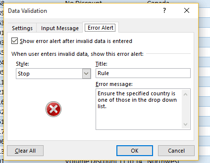
We also saw that an Error Message can be defined for when a user enters an invalid value. This is achieved via the Error Alert tab of the Data Validation dialog:

And the Error Alert tab is as follows: