Excel is more than a calculator! - Part 1

Are you getting the most out of Excel?

Excel is great at adding up numbers, but it can be used for so much more!!

• There is a rich library of functions to help create new values from stored or imported data
• There are charts and graphs that can be used to present data in a user friendly manner
• There are Pivot Tables to summarise data
• You can relate data on worksheets and carry out lookups
• Easy to use table layouts help to make data clear
• You can record macros to automate repetative tasks
• Filtering makes it easy to restrict views to relevant data
• Sorting enables you to view your data in any order you choose
• Conditional formatting enables different effects and colours to be defined based on cell values
• You can add forms and drop down boxes to your worksheets
• There are numerous add-ins to extend the data anlysis capabilities: PowerView, PowerPivot

In part 1 of this Excel blog we look at the following:

• COUNTIFS Function
• VLOOKUP Function
• A ListBox Control
• Table Formatting

Excel ListBox Control

We are going to add a ListBox control to a workbook to provide a drop down list of months to choose from:

A ListBox will return a number representing the position of the choice selected. Above we can see that January has been selected in the ListBox and the value 1 has been returned to the cell C1. ( A VLOOKUP function has been used to derive the monthname from the month number – we will see this later).

Before we configure the ListBox control we will need a lookup table that holds all the values we wish to display in the ListBox. We have this in cells I3 to J14 a shown below:

A ListBox can be added via the Developer Ribbon. If you don’t have the Developer Ribbon this can be added via File – Options – Customize Ribbon:

Select the Insert drop down on the Developer Ribbon:

The fourth icon from the left is the ListBox control so click on this to add the ListBox. Having clicked on the icon move to the workbook position and size the rectangular area for the ListBox.

To configure the ListBox right click on the ListBox (you may need to do this twice) and select Format Control from the pop up menu.

The first tab to be displayed is the Control Tab which you complete by providing the cell range containing the drop down list values and the cell to return the selected value to:

In this example we provide the range of cells containing just the month names, and the result will be returned to cell C1.

There are further customisations that can be made to the ListBox, but it will now work, providing a list of month names.

Excel VLOOKUP Function

We saw in the ListBox example that cell B1 derives a month name from the number returned by the ListBox Control. Before entering the VLOOKUP function we will need a “database” containing the value we will be looking up and the value we will be returning. One thing that is very important for VLOOKUP and HLOOKUP functions is that the lookup column of the database is sorted, or odd results will occur.

Our database in this example is in the cells I3 to J14.

=VLOOKUP(C1,I3:J14,2)

C1 is the cell containing the value we are looking up.

I3:J14 is the database (first column is the sorted lookup values)

2 is the column number to return a value from on finding a match in the first column.

Excel Table Formatting

Below is a a data set that has not been formatted in any way:

Excel provides a very simple Table Formatting utlity. It is located on the Home Ribbon in the Styles section and is called Format as Table:

Clicking on the arrow for Format as Table shows the following:

Choose a style and you will then be asked to confirm the range of cells containing your table data, including the column headings row.

The colour and border formatting will be applied to your data and filter drop downs will be added to the column heading cells.

Excel COUNTIFS Function

The COUNTIFS function enables selective cells to be counted. Cells are counted if multiple conditions are true.

In the following example we will use the previous table of data to count the number of female and male race entrants who entered a race in a selected month. There are two conditions in this example:

• Gender
• Month of entry

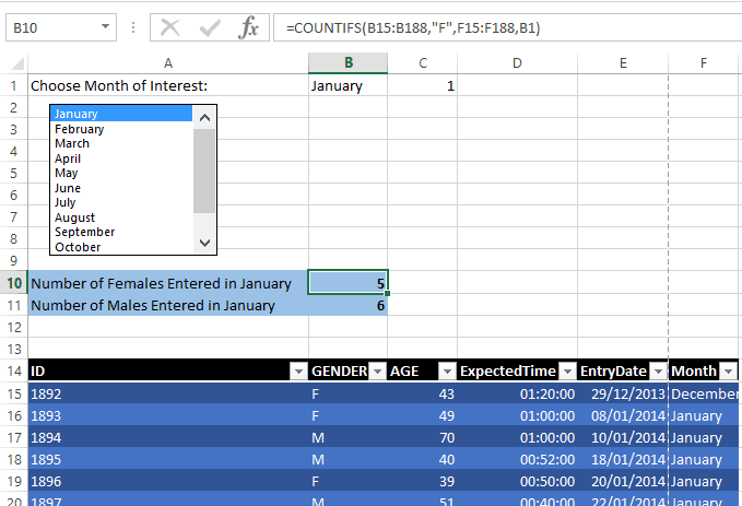
In the following screen shot we can see that the COUNTIFS has two pairs of arguments, one for each condition:

Let’s look at the formula:

=COUNTIFS(B15:B188,"F",F15:F188,B1)

B15:B188 is the range of cells containing the Gender value for a race entrant.

“F” is the gender value we are looking to match in range B15:B188.

F15:F188 is the range of cells containing the Month of race entry

B1 is the cell containing the month value we are interested in (in this example January).

The formula for the number of males is similar:

=COUNTIFS(B15:B188,"M",F15:F188,B1)

As an aside the Month of race entry is also dereived from a formula. Cell F16 contains the following:

=VLOOKUP(MONTH(E16),$I$3:$J$14,2)

It looks up the month number of cell E16 in the database in cells I3:J14 (using absolute cell references so that the range is preserved when the formula is copied down the column!) and column 2 (the month name) is the column returned from the matchinbg row in the database.

Look out for Part 2 of this blog!

If you would like to learn more about working with Excel take a look at our Excel Training Courses.