Linux - Disk Partitioning & Logical Volume Manager (LVM)

Linux Partitioning & Logical Volume Manager (LVM)

Linux, Disks and Partitions

Linux supports direct raw disk usage and Logical Volume Management to facilitate file system and swap resources. The Linux Logical Volume Manager (LVM) provides software support for concatenated, striped and mirrored logical volumes similar to those offered by hardware RAID solutions.

As Linux is installed on PC based systems it has in the past been constrained slightly by the  Master Boot Record (MBR) interface supported by motherboards.

Under MBR constraints PC systems can have a maximum of four physical partitions on a disk, configured as up to 4 primary partitions or up to 3 Primary Partitions and 1 Extended Partition. An Extended Partition can be logically partitioned further into Logical Partitions and this caters for scenarios that require more than 4 partitions from one disk.

• Where an entire disk is used for a file system or swap resource a single Primary Partition would be created.

Traditional UNIX systems frequently separated key subsets of Operating System files and directories into different file systems, which can then be mounted on to empty directories in a parent file system (often the root file system which is the core Operating System file system and is mounted on /). This is a little bit like having separate mapped drives for separate file systems in a Windows based system. Linux systems adopt this traditional UNIX convention too. For example it is common for the following pathnames to be mount points for separate file systems:

• /home
• /opt
• /var

In addition to the above at least one partition is required as a swap resource (part of the virtual memory model - similar to a Pagefile in Windows) and business data might also be isolated in separate file systems.

Each file system and swap resource will exist on a separate partition or logical volume

So as you can see with just /, /home, /opt and /var we have already exceeded 4 partitions with 4 file systems and 1 swap resource. If we separate other areas of business data then we have exceeded the limit of 4 even further and under MBR support we would need to create an Extended Partition on the disk to enable us to create Logical Partitions, and thus exceed 4 separate file systems and a swap resource.

Modern motherboards support Unified Extensible Firmware Interface (UEFI) instead of BIOS for setting up hardware and loading and starting the Operating system. UEFI systems will support GUID Partition Table (GPT), which caters for many more than four partitions, in theory the number of partitions is unlimited. GPT is gradually replacing MBR. Partition sizes can also be much bigger in GPT systems.

Linux can work with GPT even if the motherboard does not support UEFI and only offers BIOS.  GRUB 2, the boot loader used with more recent Linux systems such as Centos and RedHat 7, supports GPT.

You can check if your server supports EFI or BIOS with the following commands:

The above example was run on a BIOS based system.

The examples in this text are from a CentOS 7 system,  but the commands and processes are exactly the same in CentOS 6 (and RedHat 6 and 7).

Partitioning Disks in Linux

As described above it is dependent upon whether you are using MBR or GPT how you initially partition the disks. There are a number of partitioning tools available in Linux:

• fdisk
• gdisk
• parted

If you are using a BIOS MBR system then you can use fdisk to partition the disk.

If you are using a UEFI GPT system or have GRUB 2 as the boot loader you can use gdisk to partition the disk.

The third tool, parted, can be used to partition both MBR and GPT systems.

Generally use fdisk for drives that are less than 2TB (MBR) and either parted or gdisk for disks greater than 2TB.

The following screen shot shows an example of gdisk with an MBR disk. Only an MBR partition  table is found:

Notice that we have used gdisk here to view an MBR disk. You should use fdisk to make changes to an MBR partition table.

The following screen shot shows that the underlying server is a BIOS based system (MBR: protective), but the disk has partitioned as a GPT disk:

The following screen shot shows the output from parted for the partition layout on an MBR system (partition table: msdos):

The following screen shot shows the output from parted for the partition layout on a GPT system (partition table: gpt):

Creating Partitions with parted

The parted command takes a device pathname as an argument.

Every physical disk that is added to a Linux system will be allocated a device name. The first disk is known as sda, the second as sdb, the third as sdc and so on.

In the examples we will be seeing there are four disks present in the Linux server and their device names are:

/dev/sda

/dev/sdb

/dev/sdc

/dev/sdd

The following example enters parted with the /dev/sdc physical disk.

Typing help at the (parted) prompt displays the available commands in parted.

Before any partitions can be created the partition table type must be specified (msdos or gpt – msdos is MBR). This is done with the mklabel command:

We have specified GPT in this example.

To create partitions the mkpart command is used:

mkpart prompts for a name for the partition (this is just a label and serves no structural purpose, but it can be helpful in identifying the purpose of a partition), a starting offset and an end offset (you can specify the unit with the value as in 10GB).

The above example has created a GPT partition table with one partition at the start of the disk and 10GB in size.

We now create a second partition of the same size. The start offset is 10GB into the disk.

 A further three partitions are created and the resulting partition table is shown below:

There is a unit command that enables you to view the partition layout in a different unit. Viewing the partition table in sectors will show that parted does not allow overlaps and adjusts the start and end points accordingly to avoid overlaps:

So we now have five partitions, each of approximately 10GB in size. The total disk capacity is 136GB so we still have plenty of space currently unassigned to partitions.

Once the available disks have been partitioned the partitions can be used by Linux.

Each partition created is assigned a device name. For the example above we will have the following device names available:/dev/sdc1

/dev/sdc2

/dev/sdc3

/dev/sdc4

/dev/sdc5

Linux Logical Volume Manager (LVM)

Partitions are created from Physical Disks and Physical Volumes (PVs) are created from Partitions.

A Physical Disk can be allocated as a single Physical Volume spanning the whole disk, or can be partitioned into multiple Physical Volumes. 

Physical Volumes can be used individually to create file system and swap resources or can be used by the Logical Volume Manager to create Logical Volumes which can in turn implement RAID capabilities for improved performance and fault tolerance.

When PVs are under the control of LVM they can be grouped into Volume Groups (VGs).

Physical Volumes are divided into Physical Extents(PEs) and the partition size for all Physical Volumes in the same Volume Group is identical. Physical Extent size is 4MB. An extent is the minimum amount by which a Logical Volume may be increased or decreased in size.

Physical Partitions from the Physical Volumes in a Volume Group can be grouped together to form a Logical Volume (LV).

The Logical Volume can then be used for a file system, swap device or raw partition for an application such as Oracle.

Creating a Physical Volume

 A Physical Volume is created from a partition using the pvcreate command:

This example shows five Physical Volumes being created.

A Physical Volume has an LVM Label placed in the second sector of a disk by the pvcreate command. The LVM Label identifies the device as a LVM Physical Volume (PV). This label can actually be placed in any of the first 4 sectors of the Physical Disk as the first four sectors are all searched for an LVM label during the boot process. 

The reason for placing the LVM Label in the second sector is that the first sector is used for the legacy MBR (Master Boot Record). For backwards compatibility even though the MBR has been superseded by the more flexible GPT (GUID Partition Table) the first sector is reserved for MBR and the second sector for GPT.  A duplicate copy of a GPT is also stored at the end of the disk.

If using a whole disk device for a physical volume, the disk must have no partition table. The partition table can be erased using the dd command to zero out the first sector of the disk which is where the partition table is stored.

We can list the available PVs with the pvdisplay and pvscan commands.

Before creating PVs:

After creating PVs:

Creating a Volume Group

Now that we have some PVs we can create a Volume Group (VG) and add some PVs to it.

To create a Volume Group we use the vgcreate command:

The example above shows three arguments being passed to the vgcreate command:

• A name for the VG
• Two device pathnames for Physical Volumes (of identical size)

 If we now display information about the PVs we see the following:

We now see all five of the sdc PVs listed in the pvscan output.

The pvdisplay command now shows more information for the two PVs added to the SalesVG VG:

We can se that these two PVs belong to the SalesVG VG and that an Extent Size of 4MB has been assigned. We can also see that no space has currently been allocated from either of these PVs. We have not created any Logical Volumes yet.

 We can display information about VGs using the vgscan and vgdisplay commands:

Creating Logical Volumes

 Now that we have a Volume Group we can start creating Logical Volumes (LVs). There are three types of Logical Volume Supported:

• Linear
• Mirror
• Stripe

Linear LVs are sometimes described as Concatenated LVs. PVs are filled up sequentially rather than in parallel. So if a VG was comprised of 4 PVs and a single linear LV was created using the whole VG resource the first PV would be populated and then the second, then the third and then the fourth.

 Mirrored LVs provide fault tolerance through one or more replicas. A minimum configuration would be a two mirror LV. Each mirror would be made up from Physical Extents (totalling the specified size of the LV) on different PVs. If one mirror were to fail the good mirror would still be available enable the file system or swap device contained within it to remain in operation.

 Striped LVs provide improved performance by distributing data across multiple PVs. A stripe unit defines how much data is written to each PV in one go and writes are alternated between the PVs.

 Logical Volumes are created using the lvcreate command.

Creating a Striped Logical Volume

 In the following example we will create a two stripe (-i2) Striped LV called SalesLV1. The strip unit size is 64KB and the volume size is 5G (2.5G from each of PVs selected).

The SalesVG Volume Group only has two Physical Volumes allocated to it so the striped Logical Volume will be striping across both disks.

Creating a Mirrored Logical Volume

In the following example we create a two mirror LV called SalesLV2. The mirror volume has one mirror meaning that there will be two replicas of the data and the volume size is 5G which means that there will be two replicas of 5G size.

We have not specified which PVs to use so LVM will select two PVs with available Physical Extents. It is possible to specify which PVs to take Physical Extents from. The SalesVG Volume Group only has two Physical Volumes allocated to it so both will be used for a replica here.

Displaying Information About Logical Volumes

 The lvdisplay and lvscan commands can be used to display information about Logical Volumes.

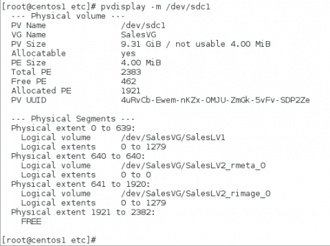
To find out which Physical Volumes Logical Volumes have data on (as if not specified on creation Physical Extents can be allocated from any PV in the VG that have adequate free space) you can use the -m option with the pvdisplay command.

The above screen shot shows that PV /dev/sdc1 contains data from two LVs - SalesLV1 and SalesLV2. We can also see that for a mirrored LV (SalesLV2) a Physical Extent is also allocated for Mirror metadata.